5. 3D Niche Modeling with the GLM Algorithm

Introduction

In this vignette, I will focus on demonstrating a basic workflow for generating and projecting a 3D ecological niche model using a generalized linear model, incorporating voluModel tools.

Here are the packages you will need.

library(voluModel) # Because of course
library(dplyr) # For occurrence data filtration

## 
## Attaching package: 'dplyr'

## The following objects are masked from 'package:stats':
## 
##     filter, lag

## The following objects are masked from 'package:base':
## 
##     intersect, setdiff, setequal, union

library(ggplot2) # For fancy plotting
library(terra) # Now being transitioned in

## terra 1.7.78

library(sf) # Now being transitioned in

## Linking to GEOS 3.11.0, GDAL 3.5.3, PROJ 9.1.0; sf_use_s2() is TRUE

library(viridisLite) # For high-contrast plotting palettes

Data Inputs

First thing’s first. Distributional models are based on coordinates of species’ occurrences. Here is an example dataset of Steindachneria argentea, Luminous Hake, using data downloaded via R (R Core Team, 2020) from GBIF (Chamberlain et al., 2021; Chamberlain and Boettiger, 2017) and OBIS (Provoost and Bosch, 2019) via occCite (Owens et al., 2021).

occs <- read.csv(system.file("extdata/Steindachneria_argentea.csv", 
                             package='voluModel'))
summary(occs$depth)

##    Min. 1st Qu.  Median    Mean 3rd Qu.    Max.    NA's 
##     0.0     0.0   117.0   184.9   353.2  2067.5     113

boxplot.stats(occs$depth)

## $stats
## [1]   0.0   0.0 117.0 354.5 676.5
## 
## $n
## [1] 188
## 
## $conf
## [1]  76.14978 157.85022
## 
## $out
## [1] 2067.5

Based on this information and what we know about the biology of Luminous Hakes and how these occurrence data are collected, I am going to remove occurrences that have a depth of 0, as well as the extreme depth outlier, since these look like either collections of individuals that were not in situ or errors of some kind.

occsClean <- occs %>% 
  dplyr::select(decimalLongitude, decimalLatitude, depth) %>%
  dplyr::distinct() %>% 
  filter(dplyr::between(depth, 1, 2000))
head(occsClean)

##   decimalLongitude decimalLatitude  depth
## 1        -54.90000        7.450000 260.50
## 2        -54.08333        7.666667 450.00
## 3        -54.08333        7.666667 450.00
## 4        -56.87500        7.741667 365.76
## 5        -80.43333        9.300000  82.00
## 6        -59.78330        9.683300 274.00

ggplot(occsClean, aes(x = 1, y=depth)) +
  geom_violin(fill="yellow", ) +
  theme_classic(base_size = 15) +
  theme(axis.title = element_blank(),
        text = element_text(family = "Arial"),
        axis.text = element_text(size = rel(1.1))) +
  ggtitle("Depth") +
  geom_boxplot(width=0.1)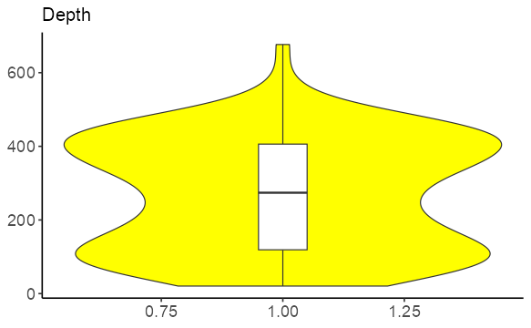

Next, we load two environmental datasets from the World Ocean Atlas (Garcia et al., 2019): temperature (Locarnini et al., 2018) and apparent oxygen utilization (Garcia et al., 2019). I have chosen these variables for simplified illustrative purposes–we recommend you explore additional variables from the World Ocean Atlas and other sources. These data are supplied by the World Ocean Atlas as point shapefiles; the version supplied here has been cropped between -110 and -40 longitude and between -5 and 50 latitude to make it more memory-efficient. For more details on how to process environmental data, see the raster data tutorial. Temperature processing is shown below for illustrative purposes.

# Temperature
td <- tempdir()
unzip(system.file("extdata/woa18_decav_t00mn01_cropped.zip", 
                  package = "voluModel"),
      exdir = paste0(td, "/temperature"), junkpaths = T)
temperature <- vect(paste0(td, "/temperature/woa18_decav_t00mn01_cropped.shp"))

# Creating a SpatRaster vector
template <- centerPointRasterTemplate(temperature)
tempTerVal <- rasterize(x = temperature, y = template, field = names(temperature))

# Get names of depths
envtNames <- gsub("[d,M]", "", names(temperature))
envtNames[[1]] <- "0"
names(tempTerVal) <- envtNames
temperature <- tempTerVal

Pre-processed apparent oxygen utilization is loaded from an .tif file for speed.

oxygenSmooth <- rast(system.file("extdata/oxygenSmooth.tif", 
                                 package='voluModel'))

# Change names to match temperature
names(oxygenSmooth) <- names(temperature)

Sampling data for model generation

The first step is down-sampling the occurrence data so that there is only one occurrence per voxel (the 3D equivalent of a pixel) of environmental data. We do this to avoid over-fitting the model due to biased sampling. The resampled points are centered in each voxel.

# Gets the layer index for each occurrence by matching to depth
layerNames <- as.numeric(names(temperature))
occsClean$index <- unlist(lapply(occsClean$depth, FUN = function(x) which.min(abs(layerNames - x))))
indices <- unique(occsClean$index)

# Downsamples occsClean in each depth layer
downsampledOccs <- data.frame()
for(i in indices){
  tempPoints <- occsClean[occsClean$index==i,]
  tempPoints <- downsample(tempPoints, temperature[[1]], 
                           verbose = FALSE)
  tempPoints$depth <- rep(layerNames[[i]], times = nrow(tempPoints))
  downsampledOccs <- rbind(downsampledOccs, tempPoints)
}

occsClean <- downsampledOccs

print(paste0("Original number of points: ", nrow(occs), "; number of downsampled occs: ", nrow(occsClean)))

## [1] "Original number of points: 301; number of downsampled occs: 82"

land <- rnaturalearth::ne_countries(scale = "small", returnclass = "sf")[1]
pointCompMap(occs1 = occs, occs2 = occsClean, 
             occs1Name = "Original", occs2Name = "Cleaned", 
             spName = "Steindachneria argentea", 
             land = land, verbose = FALSE)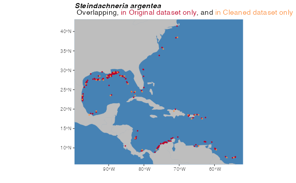

Next, we generate a sampling region for the model based on occurrence points. Note that ideally when you’re modeling you would carefully curate this background sampling region to make sure it truly approximates the area accessible to the species you are modeling. If you write the shapefile to disk, you can open and edit it in any GIS software you choose, if you have reason to believe marineBackground() falls short of estimating the true accessible are for a species. For more information, see the environmental data processing tutorial.

backgroundSamplingRegions <- marineBackground(occsClean, buff = 1000000)
crs(backgroundSamplingRegions) <- crs(land)
plot(backgroundSamplingRegions, border = F, col = "gray",
     main = "Points and Background Sampling",
     axes = T)
plot(land, col = "black", add = T)
points(occsClean[,c("decimalLongitude", "decimalLatitude")], 
       pch = 20, col = "red", cex = 1.5)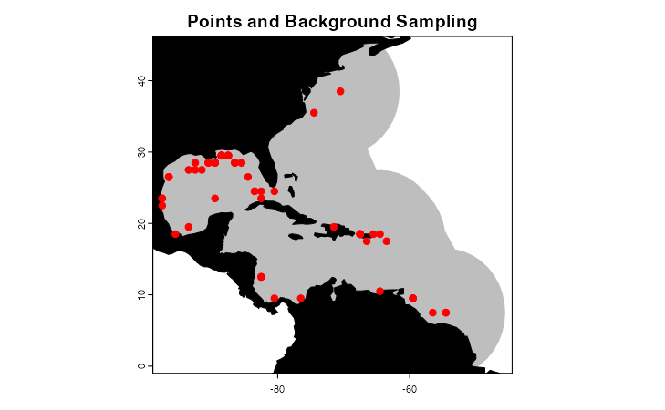

Finally, we need to draw the environmental variable data that will be used to generate the ecological niche model, from presence voxels as well as from the background sampling region. First, we sample environmental data for occurrences and add a “response” column filled with 1s, signifying these are considered “presences”.

# Presences
oxyVals <- xyzSample(occs = occsClean, oxygenSmooth)

## Using decimalLongitude, decimalLatitude, and depth
##  as x, y, and z coordinates, respectively.

tempVals <- xyzSample(occs = occsClean, temperature)

## Using decimalLongitude, decimalLatitude, and depth
##  as x, y, and z coordinates, respectively.

vals <- cbind(occsClean, oxyVals, tempVals)
colnames(vals) <- c("decimalLongitude", "decimalLatitude", "depth", "AOU", "Temperature")
vals <- vals[complete.cases(vals),]
row.names(vals) <- NULL
occsWdata <- vals

# Add response as a column
occsWdata$response <- rep(1, times = nrow(occsWdata))

Then, we generate background data by drawing occurrences from the XY extent of the background shapefile and from user-specified depths from 5 to 800m. Background points intersecting with occurrences are not returned. Then the environmental data at each background coordinate are drawn and stored in their own data object, and the “response” column is added and filled with 0s, signifying that these are to be considered “absences” when training the model.

# Background
backgroundVals <- mSampling3D(occs = occsClean, 
                              envBrick = temperature, 
                              mShp = backgroundSamplingRegions, 
                              depthLimit = c(5, 800))

## Using decimalLongitude, decimalLatitude, and depth
##  as x, y, and z coordinates, respectively.

oxyVals <- xyzSample(occs = backgroundVals, oxygenSmooth)

## Using decimalLongitude, decimalLatitude, and depth
##  as x, y, and z coordinates, respectively.

tempVals <- xyzSample(occs = backgroundVals, temperature)

## Using decimalLongitude, decimalLatitude, and depth
##  as x, y, and z coordinates, respectively.

vals <- cbind(backgroundVals, oxyVals, tempVals)
colnames(vals) <- c("decimalLongitude", "decimalLatitude", "depth", "AOU", "Temperature")
vals <- vals[complete.cases(vals),]
row.names(vals) <- NULL
backgroundWdata <- vals

# Add response as a column
backgroundWdata$response <- rep(0, times = nrow(backgroundWdata))

Generalized linear model

If you are concerned about overfitting the model because you generated a lot more background points than presence points, you can sample from the background data however you think is logical. The example below samples 100 times the number of occurrence points from the background, weighted by distance form the suitable centroid of occurrence points. That is, the more environmentally-different a background point is from an occurrence point, the more likely it is to be sampled. This is helpful for GLMs, because background points are interpreted as “absences” unlike methods like Maxent, where sampling the most dissimilar background may more likely lead to an over-fit model.

# Sample background points weighted by distance from centroid of occurrence environments
suitableCentroid <- apply(occsWdata[,c("Temperature", "AOU")], 
                          MARGIN = 2, FUN = mean)
backgroundWdata$distance <- apply(backgroundWdata[,c("Temperature", "AOU")], MARGIN = 1, 
                                  FUN = function(x) dist(rbind(suitableCentroid, x)))
backgroundWdata$sampleWeight <- (backgroundWdata$distance - 
                                 min(backgroundWdata$distance))/(max(backgroundWdata$distance)-
                                                                 min(backgroundWdata$distance))
sampleForAbsence <- sample(x = rownames(backgroundWdata), 
                           size = nrow(occsWdata) * 100, 
                           prob = backgroundWdata$sampleWeight)
backgroundWdata <- backgroundWdata[match(sampleForAbsence, 
                                         rownames(backgroundWdata)),]

Then we unite the presence and absence data into a single data object.

# Unite datasets
datForMod <- rbind(occsWdata, backgroundWdata[,colnames(occsWdata)])
rm(suitableCentroid, sampleForAbsence, backgroundWdata, occsWdata)

With the data cleaned, formatted and united into a single data.frame, generating a generalized linear model is very simple. How does it look?

glmModel <- glm(formula = response ~ Temperature *  AOU, 
                  family = binomial(link = "logit"),  data = datForMod)
summary(glmModel)

## 
## Call:
## glm(formula = response ~ Temperature * AOU, family = binomial(link = "logit"), 
##     data = datForMod)
## 
## Coefficients:
##                   Estimate Std. Error z value Pr(>|z|)    
## (Intercept)     -2.7164112  1.3519477  -2.009  0.04451 *  
## Temperature     -0.1421546  0.0640905  -2.218  0.02655 *  
## AOU             -0.0281869  0.0101987  -2.764  0.00571 ** 
## Temperature:AOU  0.0031726  0.0007086   4.477 7.57e-06 ***
## ---
## Signif. codes:  0 '***' 0.001 '**' 0.01 '*' 0.05 '.' 0.1 ' ' 1
## 
## (Dispersion parameter for binomial family taken to be 1)
## 
##     Null deviance: 291.73  on 2625  degrees of freedom
## Residual deviance: 254.48  on 2622  degrees of freedom
## AIC: 262.48
## 
## Number of Fisher Scoring iterations: 8

Now we project the model back into geographic space; at this stage, the niche model is being used to model the geographic distribution of putative suitable habit for Luminous Hake (an ENM becomes an SDM).

layerNames <- as.numeric(names(temperature))
index <- seq(from = match(min(datForMod$depth), layerNames), 
             to = match(max(datForMod$depth), layerNames), by = 1)
depthPred <- NULL
for(j in index){
  depthPreds <- c(temperature[[j]], oxygenSmooth[[j]])
  crs(depthPreds) <- "+proj=longlat +ellps=WGS84 +datum=WGS84 +no_defs"
  names(depthPreds) <- c("Temperature", "AOU")
  depthPred[[j]] <- mask(predict(depthPreds, glmModel), backgroundSamplingRegions)
  depthPred[[j]] <- crop(depthPred[[j]], backgroundSamplingRegions)
  names(depthPred[[j]]) <- layerNames[[j]]
}
glmPred <- rast(depthPred[!unlist(lapply(depthPred, FUN = function(x) is.null(x)))])

And here’s what the SDM looks like threshholded to presences and absences; raw ENM suitability values above the threshold value become presences, values below the threshold become absences. This is useful in a variety of applications, including, but not limited to visualizing the model. In this case, the threshold is the bottom tenth percentile of suitability scores at occurrences. What this means is that we are interpreting about 10% of the occurrence points to be erroneous. It is important to remember that there are MANY different thresholds you may choose based on your dataset and the goals of your analysis. Try to choose wisely.

glmThreshold <- quantile(xyzSample(datForMod[datForMod$response == 1,
                                             c("depth", "decimalLongitude", "decimalLatitude")], 
                                   glmPred), .1, na.rm = T)[[1]] # MS90

## Using decimalLongitude, decimalLatitude, and depth
##  as x, y, and z coordinates, respectively.

glmThresholded <- glmPred > glmThreshold
rclMatrix <- matrix(c(NA, NA, 0), ncol = 3, byrow = TRUE)
glmThresholded <- classify(glmThresholded, rclMatrix, include.lowest = T)

plotLayers() plots a transparent layer of suitable habitat for each depth layer. The redder the color, the shallower the layer, the bluer, the deeper. The more saturated the color, the more layers with suitable habitat. Here, I am plotting suitability from 0m to 800m, the depth range of occurrences used to train the envelope model.

plotLayers(glmThresholded, 
          land = land, landCol = "black",
          title = "Areas of suitable habitat for \n Luminous Hake, 5m to 800m")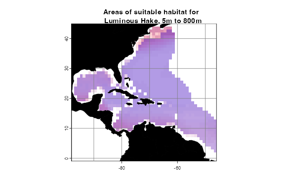

Of course, this just a starting example. We welcome submissions from the community for examples of other types of models you would like to see. Submit your suggestions as issues here.

Cropping out extreme extrapolation

Sometimes ecological models fail to extrapolate realistically when they are projected into environments that are not well-represented by the set of conditions used to calibrate the model (Owens et al, 2013). One convenient way to estimate extrapolation is via the Multivariate Environmental Suitability Surface (MESS; Elith et al. 2010). voluModel has a function, MESS3D(), which calculates MESS for each depth layer in a projection dataset (supplied to the function as a named list of RasterBrick objects used for the model projection).

# Prepare environmental data
layerNames <- as.numeric(names(temperature))
datForMod$index <- unlist(lapply(datForMod$depth, FUN = function(x) which.min(abs(layerNames - x))))
indices <- unique(datForMod$index)

projList <- list("AOU" = oxygenSmooth[[min(indices):max(indices)]], 
                 "Temperature" = temperature[[min(indices):max(indices)]])

# Calculate MESS
messBrick <- MESS3D(calibration = datForMod, projection = projList)

Now I will calculate two SpatRaster objects. In the first, extrapolation, MESS values zero and below (i.e. signalling extrapolation) will be reclassified as 1, which will allow me to easily map where extrapolation is occurring.

# Reclassify MESS 
extrapolation <- 0 >= messBrick

# Plot Extrapolation
plotLayers(extrapolation, land = land, landCol = "black", 
           title = "Areas of extrapolation according to MESS,\n 5m to 800m")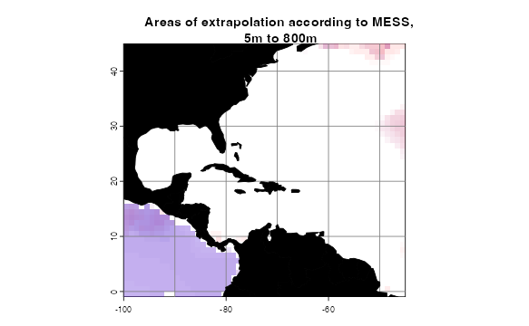

In the second RasterBrick, noExtrapolation, I reclassify the layers so that positive MESS values = 1 and MESS values less than or equal to 0 = 0. This will make plotting cropping out areas of extrapolation from the niche model projection easier. I simply multiply the thresholded GLM map by the noExtrapolation SpatRaster.

# Reclassify MESS 
noExtrapolation <- messBrick > 0

glmThreshNoExtrapolation <- NULL
for(i in 1:nlyr(noExtrapolation)){
  extrapCut <- crop(noExtrapolation[[i]], y = glmThresholded[[i]])
  croppedLayer <- glmThresholded[[i]] * extrapCut
  glmThreshNoExtrapolation[[i]] <- croppedLayer
}

glmThreshNoExtrapolation <- rast(glmThreshNoExtrapolation)

# Plot MESS
plotLayers(glmThreshNoExtrapolation, land = land, 
           landCol = "black", 
           title = "Areas of suitable habitat with no model extrapolation,\n 5m to 800m")

Tidying up

Last, we need to close the temporary directory we opened when we opened the data.

unlink(td, recursive = T)

References

Bakis Y (2021): TU_Fish. v1.1. No organization. Dataset/Occurrence. https://web.archive.org/web/20221202141213/https://bgnn.tulane.edu/ipt/resource?r=tu_fish&v=1.1 Accessed via OBIS on 2020-11-04.

Bentley A (2022). KUBI Ichthyology Collection. Version 17.80. University of Kansas Biodiversity Institute. DOI: 10.15468/mgjasg. Accessed via GBIF on 2020-10-13.

Bentley A (2022). KUBI Ichthyology Tissue Collection. Version 18.68. University of Kansas Biodiversity Institute. DOI: 10.15468/jmsnwg. Accessed via GBIF on 2020-10-13.

Buckup P A (2022). Coleção Ictiológica (MNRJ), Museu Nacional (MN), Universidade Federal do Rio de Janeiro(UFRJ). Version 157.1487. Museu Nacional / UFRJ. DOI: 10.15468/lluzfl. Accessed via GBIF on 2020-10-13.

Catania D, Fong J (2022). CAS Ichthyology (ICH). Version 150.300. California Academy of Sciences. DOI: 10.15468/efh2ib. Accessed via GBIF on 2020-10-13.

Chakrabarty P (2019). LSUMZ (LSU MNS) Fishes Collection. Version 2.2. Louisiana State University Museum of Natural Science. DOI: 10.15468/gbnym3. Accessed via GBIF on 2020-10-13.

Chamberlain S, Barve V, Mcglinn D, Oldoni D, Desmet P, Geffert L, Ram K (2021). rgbif: Interface to the Global Biodiversity Information Facility API. R package version 3.6.0, https://CRAN.R-project.org/package=rgbif.

Chamberlain S, Boettiger C (2017). “R Python, and Ruby clients for GBIF species occurrence data.” PeerJ PrePrints. DOI: 10.7287/peerj.preprints.3304v1.

Davis Rabosky AR, Cox CL, Rabosky DL, Title PO, Holmes IA, Feldman A, McGuire JA (2016). Coral snakes predict the evolution of mimicry across New World snakes. Nature Communications 7:11484.

Elith J, Kearney M, Phillips S. 2010. The art of modelling range-shifting species. Methods in Ecology and Evolution, 1, 330-342.

Espinosa Pérez H, Comisión nacional para el conocimiento y uso de la biodiversidad C (2021). Computarización de la Colección Nacional de Peces del Instituto de Biología UNAM. Version 1.9. Comisión nacional para el conocimiento y uso de la biodiversidad. DOI: 10.15468/zb2odl. Accessed via GBIF on 2020-10-13.

Frable B (2019). SIO Marine Vertebrate Collection. Version 1.7. Scripps Institution of Oceanography. DOI: 10.15468/ad1ovc. Accessed via GBIF on 2020-10-13.

Fishnet2 Portal, http://www.fishnet2.net, [Access date] Accessed via OBIS on 2020-11-04.

Froese, R. and D. Pauly. Editors. 200x. FishBase. World Wide Web electronic publication. www.fishbase.org, version (xx/200x). Accessed via OBIS on 2020-11-04.

Gall L (2021). Vertebrate Zoology Division - Ichthyology, Yale Peabody Museum. Yale University Peabody Museum. DOI: 10.15468/mgyhok. Accessed via GBIF on 2020-10-13.

García, CB, and Duarte, LO, ‘Columbian Caribbean Sea’, in J.H. Nicholls (comp.) HMAP Data Pages https://oceanspast.org/hmap_db.php Accessed via OBIS on 2020-11-04.

Garcia HE, Weathers K, Paver CR, Smolyar I, Boyer TP, Locarnini RA, Zweng MM, Mishonov AV, Baranova OK, Seidov D, Reagan JR (2018). World Ocean Atlas 2018, Volume 3: Dissolved Oxygen, Apparent Oxygen Utilization, and Oxygen Saturation. A Mishonov Technical Ed.; NOAA Atlas NESDIS 83, 38pp.

GBIF.org (24 September 2020) GBIF Occurrence Download DOI: 10.15468/dl.efuutj.

Grant S, McMahan C (2020). Field Museum of Natural History (Zoology) Fish Collection. Version 13.12. Field Museum. DOI: 10.15468/alz7wu. Accessed via GBIF on 2020-10-13.

Harvard University M, Morris P J (2022). Museum of Comparative Zoology, Harvard University. Version 162.296. Museum of Comparative Zoology, Harvard University. DOI: 10.15468/p5rupv. Accessed via GBIF on 2020-10-13.

Hendrickson D A, Cohen A E, Casarez M J (2022). University of Texas, Biodiversity Center, Ichthyology Collection (TNHCi). Version 5.175. University of Texas at Austin, Biodiversity Collections. DOI: 10.15468/h8gxdr. Accessed via GBIF on 2020-10-13.

INVEMAR. SIBM en línea: Sistema de Información sobre Biodiversidad Marina. Santa Marta: Instituto de investigaciones Marinas y Costeras José Benito Vives de Andréis,. https://siam.invemar.org.co/ Accessed via OBIS on 2020-11-04.

Locarnini RA, Mishonov AV, Baranova OK, Boyer TP, Zweng MM, Garcia HE, Reagan JR, Seidov D, Weathers K, Paver CR, Smolyar I (2018). World Ocean Atlas 2018, Volume 1: Temperature. A. Mishonov Technical Ed.; NOAA Atlas NESDIS 81, 52pp.

McLean, M.W. (2014). Straightforward Bibliography Management in R Using the RefManager Package. NA, NA. https://arxiv.org/abs/1403.2036.

McLean, M.W. (2017). RefManageR: Import and Manage BibTeX and BibLaTeX References in R. The Journal of Open Source Software.

Mertz W (2021). LACM Vertebrate Collection. Version 18.9. Natural History Museum of Los Angeles County. DOI: 10.15468/77rmwd. Accessed via GBIF on 2020-10-13.

Nakae M, Shinohara G (2018). Fish collection of National Museum of Nature and Science. National Museum of Nature and Science, Japan. Occurrence dataset DOI: 10.15468/w3dzv1 accessed via GBIF.org on yyyy-mm-dd. Accessed via OBIS on 2020-11-04.

Natural History Museum (2021). Natural History Museum (London) Collection Specimens. DOI: 10.5519/0002965. Accessed via GBIF on 2020-10-13.

National Museum of Natural History, Smithsonian Institution NMNH Fishes Collection Database. National Museum of Natural History, Smithsonian Institution, 10th and Constitution Ave. N.W., Washington, DC 20560-0193, 2007. Accessed via OBIS on 2020-11-04.

Norén M, Shah M (2017). Fishbase. FishBase. DOI: 10.15468/wk3zk7. Accessed via GBIF on 2020-10-13.

Norton B, Hogue G (2021). NCSM Ichthyology Collection. Version 22.8. North Carolina State Museum of Natural Sciences. DOI: 10.36102/dwc.1. Accessed via GBIF on 2020-10-13.

Nychka D, Furrer R, Paige J, Sain S (2021). “fields: Tools for spatial data.” R package version 13.3, <URL: https://github.com/dnychka/fieldsRPackage>.

Orrell T, Informatics Office (2021). NMNH Extant Specimen Records (USNM, US). Version 1.49. National Museum of Natural History, Smithsonian Institution. DOI: 10.15468/hnhrg3. Accessed via GBIF on 2020-10-13.

Owens H, Campbell L, Dornak L, Saupe E, Barve N, Soberón J, Ingenloff K, Lira-Noriega A, Hensz C, Myers, C, Peterson AT (2013). Constraints on interpretation of ecological niche models by limited environmental ranges on calibration areas. Ecological Modelling 263: 10-18.

Owens H, Merow C, Maitner B, Kass J, Barve V, Guralnick R (2021). occCite: Querying and Managing Large Biodiversity Occurrence Datasets_. doi: 10.5281/zenodo.4726676 (URL: DOI: 10.5281/zenodo.4726676), R package version 0.4.9.9000, (<URL: https://CRAN.R-project.org/package=occCite>).

Prestridge H (2021). Biodiversity Research and Teaching Collections - TCWC Vertebrates. Version 9.4. Texas A&M University Biodiversity Research and Teaching Collections. DOI: 10.15468/szomia. Accessed via GBIF on 2020-10-13.

Provoost P, Bosch S (2019). “robis: R Client to access data from the OBIS API.” Ocean Biogeographic Information System. Intergovernmental Oceanographic Commission of UNESCO. R package version 2.1.8, https://cran.r-project.org/package=robis.

Pugh W (2021). UAIC Ichthyological Collection. Version 3.3. University of Alabama Biodiversity and Systematics. DOI: 10.15468/a2laag. Accessed via GBIF on 2020-10-13.

R Core Team (2017). R: A language and environment for statistical computing. R Foundation for Statistical Computing, Vienna, Austria. URL https://www.R-project.org/.

Robins R (2021). UF FLMNH Ichthyology. Version 117.342. Florida Museum of Natural History. DOI: 10.15468/8mjsel. Accessed via GBIF on 2020-10-13.

Tavera L, Tavera M. L (2021). Biodiversidad de los recursos marinos y costeros entre Cartagena y el Golfo de Urabá, Caribe colombiano. Version 2.4. Instituto de Investigaciones Marinas y Costeras - Invemar. DOI: 10.15472/d2jusp. Accessed via GBIF on 2020-10-13.

UNIBIO, IBUNAM. CNPE/Coleccion Nacional de Peces. DOI: 10.15468/o5d48z. Accessed via GBIF on 2020-10-13.

Wagner M (2017). MMNS Ichthyology Collection. Mississippi Museum of Natural Science. DOI: 10.15468/4c3qeq. Accessed via GBIF on 2020-10-13.

Werneke D (2019). AUM Fish Collection. Version 8.1. Auburn University Museum. DOI: 10.15468/dm3oyz. Accessed via GBIF on 2020-10-13.

Hannah L. Owens

Carsten Rahbek