2. Processing Raster Data
Hannah L. Owens
Carsten Rahbek
2026-07-23
Source:vignettes/b_RasterProcessing.Rmd
b_RasterProcessing.RmdIntroduction
Naturally, to build 3D distribution models, one needs three-dimensionally structured environmental data. These data may come in the form of interpolated in situ measurements (e.g. NOAA’s World Ocean Atlas dataset; Garcia et al. 2018a) or as outputs from climate models, either as stand-alone ocean components or as a component of coupled atmosphere-ocean models (e.g. CCSM3, Collins et al. 2006; HadCM3, Valdes et al. 2017). Typically, these data are organized as a series of horizontal layers that are stacked by depth.
Data Inputs
First, let’s look at a relatively simple environmental variable from
the WOA: temperature (Locarnini et al, 2018). These data are supplied by
the World Ocean Atlas as point shapefiles; the version supplied here has
been cropped between -98 and -45 longitude, between -1 and 45 latitude,
and between 0 and 4,400 m in depth to make it more space-efficientf. You
can download the full dataset via the WOA website. Our first task is to
read in the shapefile as a SpatVector. Note that each row
in temperature is a set of horizontal coordinates. Each
column is a vertical position in the water column. Make sure to check
the metadata of the data you use. Different sources may use vertical
depth structures.
# Temperature
td <- tempdir()
unzip(system.file("extdata/woa18_decav_t00mn01_cropped.zip",
                  package = "voluModel"),
      exdir = paste0(td, "/temperature"), junkpaths = T)
temperature <- vect(paste0(td, "/temperature/woa18_decav_t00mn01_cropped.shp"))

# Looking at the dataset
as.data.frame(temperature[1:5,1:10])
## SURFACE d5M d10M d15M d20M d25M d30M d35M d40M d45M
## 1 23.575 23.392 22.919 22.318 21.766 21.117 20.531 19.860 19.266 18.673
## 2 23.204 22.979 22.559 22.057 21.401 20.651 19.978 19.433 18.835 18.247
## 3 23.451 23.125 22.726 22.134 21.520 20.828 20.128 19.472 18.875 18.353
## 4 23.261 22.968 22.559 22.052 21.528 20.945 20.337 19.759 19.198 18.669
## 5 22.977 22.790 22.463 22.036 21.611 21.079 20.521 20.000 19.423 18.835
# Plotting the dataset
layout(matrix(c(1, 2), ncol=2, byrow=TRUE), widths=c(4, 1))
land <- rnaturalearth::ne_countries(scale = "small",
                                    returnclass = "sf")[1]
temperatureForPlot <- temperature
crs(temperatureForPlot) <- crs(land)
ext <- ext(temperatureForPlot)
plot(temperatureForPlot, main = "Distribution of voluModel Subset\nof WOA Temperature 2018",
     pch = 20, col = "red", xlim = ext[1:2], ylim = ext[3:4], cex = .6, mar = c(2,2,3,2))
plot(land, col = "black", add = T)

# What does the WOA depth structure look like?
depths <- names(temperatureForPlot)
depths <- as.numeric(gsub(depths[-1], pattern = "[d,M]", replacement = ""))
plot(0, xlim = c(0,1), ylim = c(0-max(depths), 0), axes=FALSE, type = "n", xlab = "", ylab = "Depth Intervals (m)")
axis(2, at = 0-depths, labels = depths)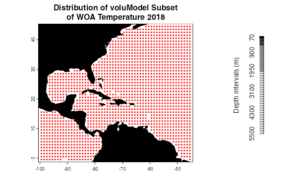
Next, we convert temperature into a SpatRaster. While we
are at it, we will generate a raster from the deepest value available
for each point. While you might call this a “bottom” raster, it is
important to note that in some cases, values are not available for the
bottom. After the SpatRaster is created, we give it the
same depth names as the columns in the SpatVector. This is
important, because voluModel uses these names as z
coordinates when handling 3D data. I am using
oneRasterPlot() from voluModel to visualize the rasters
using a uniform, high-contrast aesthetic.
# Creating a bottom raster
temperatureBottom <- bottomRaster(temperature)

# Creating a SpatRaster vector
template <- centerPointRasterTemplate(temperature)
tempTerVal <- rasterize(x = temperature, y = template, field = names(temperature))

# Get names of depths
envtNames <- gsub("[d,M]", "", names(temperature))
envtNames[[1]] <- "0"
names(tempTerVal) <- envtNames
temperature <- tempTerVal
rm(tempTerVal)

# How do these files look?
par(mfrow=c(1,2))
p1 <- oneRasterPlot(temperature[[1]], land = land, landCol = "black",
              title= "Surface Temperature (C)")

p2 <- oneRasterPlot(temperatureBottom,land = land, landCol = "black",
              title = "Bottom Temperature (C)")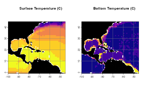
Interpolation
Next, we have a bit of a more complicated example: apparent oxygen utilization (AOU; Garcia et al, 2018b). Apparent oxygen usage is more patchily sampled than temperature (it’s generally measured from instrument casts on research cruises, and the coverage isn’t quite as dense as for temperature).
td <- tempdir()
unzip(system.file("extdata/woa18_all_A00mn01_cropped.zip",
                  package = "voluModel"),
      exdir = paste0(td, "/oxygen"), junkpaths = T)

oxygen <- vect(paste0(td, "/oxygen/woa18_all_A00mn01_cropped.shp"))

plot(oxygen, main = "Distribution of voluModel subset of WOA AOU 2018",
     pch = 20, col = "red", xlim = ext[1:2], ylim = ext[3:4], cex = .6)
plot(land, col = "black", add = T)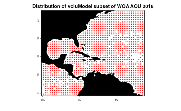
There is a workaround for this, since we can reasonably expect some
degree of spatial autocorrelation in apparent oxygen utilization. We use
the interpolateRaster() function to produce
statistically-interpolated layers using TPS() from the
fields package (this is a thin-plate spline interpolation).
Be patient–this step can take a while, although as shown here, I am
using the fastTPS() approximation, which only samples from
nearby cells to speed things up. Maybe fastTPS() will work
ok for your data, maybe it won’t. It depends on the data. For the sake
of efficiency for this example, I am going to limit this to the first 10
depth layers.
# Creating a SpatRaster vector for the first 10 depth layers
oxygen <- oxygen[,1:10] # Remove this line if you want to process the whole file
oxygen <- rasterize(x = oxygen, y = template,
                   field = names(oxygen)) #Uses same raster template as temperature

for (i in 1:nlyr(oxygen)){
  oxygen[[i]] <- interpolateRaster(oxygen[[i]], lon.lat = T, fast = T, aRange = 30) #Thin plate spline interpolation
  oxygen[[i]] <- crop(mask(x = oxygen[[i]],
                           mask = temperature[[i]]),
                      temperature[[i]])
}

# Change names to match tempT
names(oxygen) <- envtNames[1:nlyr(oxygen)]
Some environmental data rasters may also look “patchy”, possibly as
an artifact of uneven sampling. If you are confident that there should
be a strong spatial correlation in a data layer that looks “patchy”, you
can also statistically smooth it, again using TPS(), like
this:
# Smoothing tempO and saving
oxygenSmooth <- oxygen
for (i in 1:nlyr(oxygenSmooth)){
  oxygenSmooth[[i]] <- smoothRaster(oxygenSmooth[[i]], lon.lat = T) #Thin plate spline interpolation
  oxygenSmooth[[i]] <- crop(mask(x = oxygenSmooth[[i]], mask = temperature[[i]]), temperature[[i]])
}
## Warning:
## Grid searches over lambda (nugget and sill variances) with minima at the endpoints:
## (GCV) Generalized Cross-Validation
## minimum at right endpoint lambda = 0.06197414 (eff. df= 127.3 )
## Warning:
## Grid searches over lambda (nugget and sill variances) with minima at the endpoints:
## (GCV) Generalized Cross-Validation
## minimum at right endpoint lambda = 0.06197414 (eff. df= 127.3 )
## Warning:
## Grid searches over lambda (nugget and sill variances) with minima at the endpoints:
## (GCV) Generalized Cross-Validation
## minimum at right endpoint lambda = 0.06197414 (eff. df= 127.3 )
## Warning:
## Grid searches over lambda (nugget and sill variances) with minima at the endpoints:
## (GCV) Generalized Cross-Validation
## minimum at right endpoint lambda = 0.06197414 (eff. df= 127.3 )
## Warning:
## Grid searches over lambda (nugget and sill variances) with minima at the endpoints:
## (GCV) Generalized Cross-Validation
## minimum at right endpoint lambda = 0.06203537 (eff. df= 126.3499 )
## Warning:
## Grid searches over lambda (nugget and sill variances) with minima at the endpoints:
## (GCV) Generalized Cross-Validation
## minimum at right endpoint lambda = 0.06203537 (eff. df= 126.3499 )
# Change names to match tempT and save
names(oxygenSmooth) <- names(oxygen)
oxygenSmooth <- oxygenSmooth

par(mfrow=c(1,2))
p3 <- oneRasterPlot(oxygen[[1]], land = land, landCol = "black",
              title= "Surface Apparent Oxygen Utilization\n(µmol/kg), interpolated")
p4 <- oneRasterPlot(oxygenSmooth[[1]], land = land, landCol = "black",
     title = "Surface Apparent Oxygen Utilization\n(µmol/kg), interpolated and smoothed")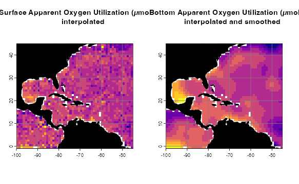
Tidying up
Last, we need to close the temporary directory we opened when we opened the data.
unlink(td, recursive = T)References
Collins WD, Bitz CM, Blackmon ML, Bonan GB, Bretherton CS, Carton JA, Chang P, Doney SC, Hack JJ, Henderson TB, Kiehl JT, Large WG, McKenna DS, Santer BD, Smith RD. (2006) The Community Climate System Model Version 3 (CCSM3) Journal of Climate, 19(11), 2122–2143 DOI: 10.1175/jcli3761.1
Garcia HE, Boyer P, Baranova OK, Locarnini RA, Mishonov AV, Grodsky A, Paver CR, Weathers KW, Smolyar IV, Reagan JR, Seidov D, Zweng MM. (2018a). World Ocean Atlas 2018 (A. Mishonov, Ed.). NOAA National Centers for Environmental Information. https://doi.org/10.25923/tzyw-rp36
Garcia HE, Weathers K, Paver CR, Smolyar I, Boyer TP, Locarnini RA, Zweng MM, Mishonov AV, Baranova OK, Seidov D, Reagan JR (2018b). World Ocean Atlas 2018, Volume 3: Dissolved Oxygen, Apparent Oxygen Utilization, and Oxygen Saturation. A Mishonov Technical Ed.; NOAA Atlas NESDIS 83, 38pp.
Locarnini RA, Mishonov AV, Baranova OK, Boyer TP, Zweng MM, Garcia HE, Reagan JR, Seidov D, Weathers K, Paver CR, Smolyar I (2018). World Ocean Atlas 2018, Volume 1: Temperature. A. Mishonov Technical Ed.; NOAA Atlas NESDIS 81, 52pp.
Nychka D, Furrer R, Paige J, Sain S (2021). “fields: Tools for spatial data.” R package version 13.3, <URL: https://github.com/dnychka/fieldsRPackage>.
R Core Team (2017). R: A language and environment for statistical computing. R Foundation for Statistical Computing, Vienna, Austria. URL https://www.R-project.org/.
Valdes PJ, Armstrong E, Badger MPS, Bradshaw CD, Bragg F, Crucifix M, Davies-Barnard T, Day JJ, Farnsworth A, Gordon C, Hopcroft PO, Kennedy AT, Lord NS, Lunt DJ, Marzocchi A, Parry LM, Pope V, Roberts WHG, Stone EJ, … Williams JHT. (2017). The BRIDGE HadCM3 family of climate models: HadCM3@Bristol v1.0. Geoscientific Model Development, 10(10), 3715–3743. DOI: 10.5194/gmd-10-3715-2017