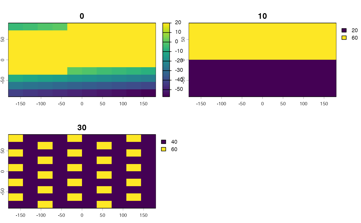
Calculate MESS

Calculates multivariate environmental similarity surface based on model calibration and projection data

MESS3D(calibration, projection)

Arguments

calibration: A data.frame of environmental variables used to calibrate an ecological niche model, one row for measurements from each voxel included in the data used to calibrate the model. Columns with names not corresponding to projection list items are ignored.
projection: A named list of SpatRaster objects for projection; names correspond to calibration column names. Each SpatRaster should have the same number of layers, corresponding to vertical depth slices.

Value

A SpatRaster vector with MESS scores for each voxel; layer names correspond to layer names of first SpatRaster vector in projection

list.

Details

MESS3D is a wrapper around MESS from the modEvA package. It calculates MESS for each depth layer. Negative values indicate areas of extrapolation which should be interpreted with caution (see Elith et al, 2010 in MEE).

Note

The calibration dataset should include both presences and background/pseudoabsence points used to calibrate an ecological niche model.

References

Elith J, Kearney M, and Phillips S. 2010. The art of modelling range-shifting species. Methods in Ecology and Evolution, 1, 330-342.

Examples

library(terra)
#> terra 1.7.71
library(dplyr)
#> 
#> Attaching package: ‘dplyr’
#> The following objects are masked from ‘package:terra’:
#> 
#>     intersect, union
#> The following objects are masked from ‘package:stats’:
#> 
#>     filter, lag
#> The following objects are masked from ‘package:base’:
#> 
#>     intersect, setdiff, setequal, union

# Create sample rasterBricks
r1 <- rast(ncol=10, nrow=10)
values(r1) <- 1:100
r2 <- rast(ncol=10, nrow=10)
values(r2) <- c(rep(20, times = 50), rep(60, times = 50))
r3 <- rast(ncol=10, nrow=10)
values(r3) <- 8
envBrick1 <- c(r1, r2, r3)
names(envBrick1) <- c(0, 10, 30)

r1 <- rast(ncol=10, nrow=10)
values(r1) <- 100:1
r2 <- rast(ncol=10, nrow=10)
values(r2) <- c(rep(10, times = 50), rep(20, times = 50))
r3 <- rast(ncol=10, nrow=10)
values(r3) <- c(rep(c(10,20,30,25), times = 25))
envBrick2 <- c(r1, r2, r3)
names(envBrick2) <- c(0, 10, 30)

rastList <- list("temperature" = envBrick1, "salinity" = envBrick2)

# Create test reference set
set.seed(0)
longitude <- sample(ext(envBrick1)[1]:ext(envBrick1)[2],
                    size = 10, replace = FALSE)
set.seed(0)
latitude <- sample(ext(envBrick1)[3]:ext(envBrick1)[4],
                   size = 10, replace = FALSE)
set.seed(0)
depth <- sample(0:35, size = 10, replace = TRUE)
occurrences <- as.data.frame(cbind(longitude,latitude,depth))

# Calibration
calibration <- lapply(rastList, FUN = function(x) xyzSample(occurrences, x)) %>% bind_rows
#> Using longitude, latitude, and depth
#>  as x, y, and z coordinates, respectively.
#> Using longitude, latitude, and depth
#>  as x, y, and z coordinates, respectively.

# Run the function
messStack <- MESS3D(calibration = calibration, projection = rastList)
plot(messStack)